Algebraic Contact Graph Routing

The Semiring Structure of Satellite Communication

In this post we will introduce a series of idempotent semirings that I have created which capture the behaviors of delay tolerant networks. These semirings allow us to use the framework of the algebraic path problem (See the prior post for an introduction to idempotent semirings and the algebraic path problem) to analyze and create routing algorithms for deep space networks and other delay tolerant networks.

To fully model a delay tolerant networn (DTN), like a deep space satellite network, we need a semiring which can encapsulate:

• Delays
• Disruptions
• Store and Forward Behavior.

In the books Path Problems in Networks and Graphs, Dioids and Semirings there are semirings which can be used to model delays and disruptions, but we will introduce a series of novel semirings which can be used to model and analyze network storage as well as delays and disruption tolerant communications.

Contact Graph Routing

Contact Graph Routing, the current algorithms and implementations of them can be read about in more detail in the papers Routing in the Space Internet and Contact graph routing in DTN space networks.

We will give a brief introduction to the problem here. We will use the contact multigraph perspective on these routing problems.

You have a set of nodes (satellites, routers, robots, ect.) \(X\), and between each pair of nodes, \(a, b \in X\), you have a set of contact windows \(C_{ab}\). A contact window is an interval \([s,e] \subseteq \mathbb R\) and a delay \(\omega \ge 0\); representing that at a time \(t \in [s,e]\) you can send a message from node \(a\) to node \(b\) and it will arrive at time \(t + \omega\). We represent contacts as pairs \(([s,e]:\omega)\).

Contact graph routing is the problem of finding a path through a contact graph to give a message the earliest arrival time possible.

For example consider the graph in figure 1. Here we have two possible routes from node \(a\) to node \(c\), either \(a \to b \to c\) or \(a \to d \to c\).

The route \(a \to b \to c\) can be used along time interval \([0,2]\) and has a total delay of \(15\), giving us potential arrival times of \([15,17]\)

The route \(a \to d \to c\) either gives us no arrival window if our nodes do not have storage capabilities, or if we are allowed to store at node \(d\) then we can send a message at any time in the interval \([0,5]\) and arrive between times \([11,12]\).

There are many ways in which we can analyse and compare these routes. We can talk about earliest arrival time, or the largest throughput of data we can get through a route, or the minimal amount of storage needed to use a route. We would like to be able to represent this routing problem algebraically in a semiring which allows us to analyze any of these potential optimization targets on our routes.

Universal Contact Semiring

I first introduced this semiring in section 2.5 of the paper Algebraic and Geometric Models for Space Networking, and since then with help from great comments from Tung Lam, Justin Curry and David Spivak this semiring has been refined to a more natural form.

Because this semiring contains as subsemirings many of the semirings used to model contact graphs we call it the universal contact semiring, here we will denote it by \(\mathcal C\).

An element of the universal contact semiring is a subset of \(\mathbb R \times \mathbb R\) where for each coordinate \((a,b)\) we have \(b \ge a\). A pair \((a,b)\) being an element of \(X \in \mathcal C\) represents being able to send a message at time \(a\) and having it arrive at time \(b\).

Delays can be modeled by having arrival times after sending time. Disruption is modelled by having missing send times. Storage can be modelled by allowing a single send time to have multiple arrival times.

For instance if we examine the element:

We have that we can send a message along link \(X\) at any time until time \(10\), and that message will arrive with a delay of \(1\) and can be stored for \(9\) units of time.

If we have two elements \(X, Y \in \mathcal C\), \(X + Y\) represents being able to use the link given by \(X\) or the link given by \(Y\). So we get:

Alternatively:

Where \(a \oplus b\) is the logical OR.

\(X *_{\mathcal C} Y\) represents taking a path allowed by \(X\) then a path allowed by \(Y\). So for a pair \((i,j)\) to be in \(X *_{\mathcal C} Y\) we need a \(k\) such that \((i,k) \in X\) and \((k,j) \in Y\). So we get:

If we write \(\otimes\) for the logical AND we can write this condition as:

This looks a whole lot like matrix multiplication, because it is! Every element of the universal contact semiring can be written as a \(\mathbb R \times \mathbb R\) boolean matrix.

We restrict \(\mathcal C\) to upper triangular matrices to avoid time travelling – a message cannot arrive before it is sent.

A contact \(([s,e]:\omega)\) can be modelled as the matrix:

Being able to store indefinitely at a node can be modelled by the storage matrix:

We can model a contact graph on a set of nodes \(X\) as an element \(A\) in \(M_X(\mathcal C)\) where

That is, we place the storage matrix on all self loops, and we take the sum of all contact matrices between nodes \(i\) and \(j\) as the edge between \(i\) and \(j\). Finding the Kleene star of the matrix \(A\) gives all possible time windows where we can communicate between nodes in our contact graph.

Working with this semiring has a notable downside – we can’t compute arbitrary elements of \(\mathcal C\). We are dealing with \(\mathbb R \times \mathbb R\) matrices, we might not be able to represent them computably, and their matrix multiplication may not be computable. There’s two approaches we could take here. We could use a discretization method like the pixel array method to do our computation with bounded error, or we could find computable subsemirings which require no discretization.

Nevada Semiring

To talk about contact graph routing we only really need the contact matrices, the storage matrix, and all of their combinations. If we have a finite number of contacts, then any element of \(A\) (the adjacency matrix for our contact graph) or its powers will be a finite sum of multiplicative words made up of contact matcies and storage matrices. To talk about these elements we just need to nicely classify the multiplicative words.

From here on out we will refer to the matrix \(X^{([s,e]:\omega)}\) using the name of the contact window, \(([s,e]:\omega)\), i.e. \(([s,e]:\omega)_{ij} = X^{([s,e]:\omega)}_{ij}\).

If we have two contacts \(([s_1,e_1]:\omega_1)\), \(([s_2,e_2]:\omega_2)\) multiplying them corresponds to composing the two contacts. This forms another contact:

Our multiplicative identity is the contact \(((-\infty, \infty):0)\).

Our storage matrix is multiplicatively idempotent, that is \(S * S = S\).

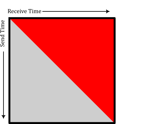
We can examine the figures we get by multiplying contacts and storages. Because we know that contacts times contacts are contacts, and storage times itself is still itself, we have two taxa of length two multiplicative words – either we multiply a contact by a storage, \(([s,e]:\omega)S\), or a storage times a contact, \(S([s,e]:\omega)\).

When we do so we see that left multiplying by a storage matrix “extends” our shapes vertically, and right multiplying by a storage matrix “extends” our shapes horizontally.

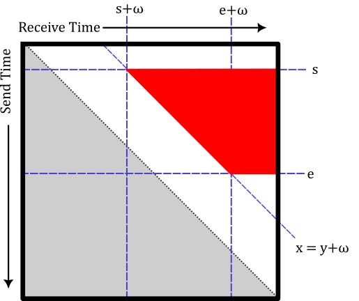
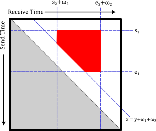
We have two taxa of length three multiplicative words. Either we can conjugate a contact by storage matrices, \(S ([s,e]:\omega) S\), or we can conjugate the storage matrix by contacts \(([s_1,e_1]:\omega_1) S ([s_2, e_2]:\omega_2)\).

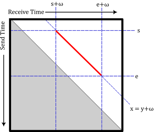
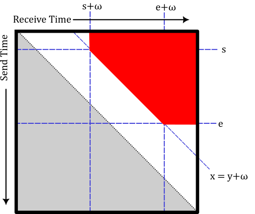
Due to the general form of contact-storage-contact matrices being that of the state of Nevada, we call a contact-storage-contact element a nevada. We denote these elements with a lower case n to avoid confusion with the state of Nevada. A nevada can be seen as the shape carved out by the five half planes:

1. \(x \ge s_2 + \omega_2\)
2. \(x \le e_2 + \omega_2\)
3. \(y \ge s_1\)
4. \(y \le e_2\)
5. \(x \ge y + \omega_2 + \omega_2\)

Where \(x\) denotes the recieve time and \(y\) denotes the send time.

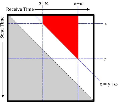
If we look back and forth between figure 6 and figure 7 quickly, we can note that the storage-contact-storage matrices can be rewritten in the form of nevadas. We call this the S-conjugation law in the nevada semiring.

From the perspective of nevadas given by the five hyperplanes we get the canonical form of a nevada.

Given a nevada \(([s_1,e_1]:\omega_1)S([s_2,e_2]:\omega_2)\) the canonical form is

There may be two nevadas with distinct delays that have the same support when seen as a matrix. In settings where the delay is relevant, and not just the availability windows we may want to work over a purely symbolic form rather than with the matrices. This symbolic form we call the nevada monoid.

These axioms are:

• Declaring what \(\emptyset\) is, and that an empty contact is empty, as well as the concatenation of \(\emptyset\) and any object
• Declaring what the multiplication of contacts is
• Saying that nevadas are equal up to canonical form
• Saying that \(S\) is multiplicatively idempotent
• Declaring the \(S\)-conjugation law as an axiom.

These relations can be summed up in three important formulas:

• The multiplication of contacts:
  
  $$([s_1,e_1] : \omega_1) * ([s_2,e_2] : \omega_2) = ([\max(s_1, s_2 - \omega_1, \min(e_1, e_2 - \omega_1)] : \omega_1 + \omega_2)$$
• The \(S\)-conjugation law:
  
  $$S * ([s,e]:\omega) * S = ((-\infty, e]:0) * S * ([s,\infty) : \omega)$$
• The canonical form:
  $$([s_1, e_1]:\omega_1)S([s_2,e_2]:\omega_2)=([s_1, \min(e_1, e_2 - \omega_1)]:0)S([\max(s_2 - \omega_1, s_1),e_2 - \omega_1]:\omega_1 + \omega_2)$$

The realization of nevadas as matrices gives us a map of monoids \(\varphi : \mathcal N \to \mathcal C\). This is not an injective map, as if we examine the nevadas

These are distinct elements in \(\mathcal N\), as they have distinct delays, but one can verify that \(\varphi(n_1) = \varphi(n_2)\).

We can use \(\varphi\) and the universal algebra isomorphism theorems to define a computable subsemiring of \(\mathcal C\).

\(\varphi\) lifts to become a semiring homomorphism \(\phi : P_{fin}(\mathcal N) \to \mathcal C\), where \(P_{fin}(\mathcal N)\) is the semiring of finite subsets of \(\mathcal N\), where addition is union and multiplication is Minkowski multiplication.

The image of \(\phi\) is a subsemiring of the universal contact semiring that we call the Store and Forward Semiring, as it is the smallest subsemiring of \(\mathcal C\) which encapsulates the store and forward behavior. We denote it \(\mathcal C_{SF} = \phi(P_{fin}(\mathcal N))\).

The isomorphism theorems give us a way to explicitly compute this semiring, as by the isomorphism theorems we know that:

Where a set of nevadas and contacts \(X_1\) is related to another \(X_2\) if and only if they have the same total support as boolean matrices. As each nevada is convex and a well defined shape we can efficiently check if two collections of nevadas have the same coverage.

This tells us that to compute in \(\mathcal C_{SF}\) we can represent each element as a finite set of nevadas and contacts. We can then perform multiplication in \(\mathcal N\), which we can do efficiently. Code implementing this semiring can be found at https://github.com/wrbernardoni/Semiring-Geometry as the CGRSemiring class.

This semiring gives us a quick way to compute the contact windows in delay tolerant networks, and by working over this semiring we can make routing decisions, and analyze potential network topographies. It gives us an algebraic method of talking about these networks – we can set up and solve equations, we can talk about underlying geometries, ect. One additional use is that it allows us to make visualization tools for these networks.

Visualizing DTN

Delay tolerant networks are strange objects that shift with time, and are not at all easy to visualize. The boolean matrices in \(\mathcal C_{SF}\) we can draw, and gain intuition about.

They give us a tool to visually see how “fragmented” a delay tolerant network is, and how “large” contact windows are.

Let \(A\) be the \(\mathcal C_{SF}\) weighted adjacency matrix of our contact graph.

To do so we create step matrices \(T_n \in M_X(\mathcal C_{SF})\). \((T_n)_{ab}\) tells us the windows in time that we can leave node \(a\) and arrive at node \(b\) in \(n\) or fewer steps. We can find these matrices as follows.

We first create an “off-diagonal” matrix \(D\):

The set of times that we can send a matrix at node \(a\) and have it arrive at node \(b\) in \(0\) steps is empty if \(a \ne b\) and it is the contact \(((-\infty, \infty):0)\) if \(a = b\), and so we define \(T_0 = 1_{M_X(\mathcal C_{SF})}\) as the identity matrix.

In \(1\) or fewer steps it is given by the matrix \(T_1 = I + D\), in \(2\) or fewer it is \(T_2 = I + D + D^2\) and in \(n \ge 2\) or fewer steps by

By plotting \((T_n)_{ab}\) we can see the windows in which we can immediately send a message from node \(a\) and have it arrive at node \(b\) in \(n\) or fewer steps.

Above we can see a demo of this visualization tool. The demo was computed on a simulated 15 by 15 Earth-Moon satellite network, centered around a proposed lunar base. Above we show a 3 by 3 slice of the network. You can see that sending a message from a proposed IOAG South satellite to the Goldstone Earth ground station has larger, less fragmented communication windows than sending a message from the IOAG South satellite to a lunar rover. This is a highly connected network, and so with a sufficient hop limit we have full coverage of the day long window – we can send and recieve a message at essentially any time – however various network topologies could increase the size of the individual windows, or reduce the hop limit required. The full output can be seen here (Warning the file is 50 Mb).

We compute the \(T_n\) matrices instead of just the cumulants \(A^{(n)}\) as the \(T_n\) matrices line up closer to our intuition on what the contact windows “should” be. The \(T_n\) matrices tell us the times that a message can immediately leave our first node and first arrive at another – whereas in the cumulants we could store on the initial or final node. The cumulants tell us what times we could drop a message off at our sending node and pick it up at our recieving node, but it might need to sit at the first or last node for a bit.

Polyhedral Contact Semiring

The store and forward semiring assumes that along a contact we have a single fixed delay. If our nodes are moving slowly relative to the length of our contact windows then this is not a bad assumption to make, and will give an accurate approximation of the delays in our network. If our nodes are moving quickly relative to the length of our contact windows then the delays may wildly vary during a fixed contact window. We can approximate this in \(\mathcal C_{SF}\) by breaking contacts into smaller locally constant delay regions – but it could be beneficial to have a computable semiring which can handle non-constant delays.

Our next computable subsemiring does just that. We will assume that the support of our matrices are finite unions of polyhedra. This forms a significantly larger subsemiring of the universal contact semiring that we call the Polyhedral UCS, and denote as \(\mathcal C_P\).

This subsemiring has a computable multiplication, as we will show that the multiplication of two polyhedral basics is another polyhedral basic, and can be computed with a computational geometric algorithm.

Let \(A\) and \(B\) be polyhedral basics with polygons \(P_A\) and \(P_B\) respectively. The multiplication \(AB\) can be found as follows.

First we create two 3D polyhedral shapes, \(C_A\) and \(C_B\) as follows:

As these are polyhedra there exist efficient algorithms to calculate \(C_A \cap C_B\). We note that we can describe the product \(AB\) as

or equivalently:

In other words, the support of \(AB\) is a skewed version of the shadow of \(C_A \cap C_B\) on the \(e_1-e_3\) plane. So to find \(AB\) we just need to:

1. Compute \(C_A \cap C_B\)
2. Compute the shadow of \(C_A \cap C_B\) on the \(e_1 - e_3\) plane: so we apply the transformation
   \(\begin{bmatrix}1 & 0 & 0\\ 0 & 0 & 1\end{bmatrix}\)
3. Skew the shadow with the transformation
   \(\begin{bmatrix}1 & 0 \\ 1 & - 1\end{bmatrix}\)

That transformed shadow is the support of \(AB\).

To compute arbitrary multiplication in \(\mathcal C_P\) we decompose our two elements into polyhedral basics and do the above process between each pair of polyhedral basic.

We note two extensions of this.

1. This algorithm works even if we do not restrict to upper triangular matrices – so we can use this to form a computable subsemiring of \(M_{\mathbb B}(\mathbb R)\) rather than just \(\mathcal C\)
2. We can do this for any shapes that we can compute intersections and projections of. So our support does not need to just be polygons, they could be shapes defined by splines, or any other graphic that can be efficiently computed.

These semirings give us computable methods of determining the largest communication windows possible. They allow us to answer the question “when can a message be sent through this network”. We can extend each of these semirings further.

If we had prices attached to each of our contacts, or other cost functions given by a semiring \(S\), we could form weighted contact semirings by examining upper triangular matrices in \(M_{\mathbb R}(S)\) and the corresponding subsemirings.

This framework allows us to use all of the methods and theory developed behind the algebraic path problem and throw them at the problems that appear in delay tolerant networks.